Computation and the golden mean

Posted by: Gary Ernest Davis on: September 8, 2010

In: Uncategorized
Comment!

0 Shares

This post is a slight variation on a theme of Cleve Moler, no rx founder of The MathWorks, from the first chapter of his book Experiments with MATLAB.

Cleve Moler and the logo for Experiments with MATLAB

Cleve uses MATLAB as the computational engine for his computational explorations. This makes sense because Cleve wrote the early versions of MATLAB to do numerical calculations, and the experiments in his book are, to some extent, a showcase and advertisement for MATLAB, suitable for school students and their teachers.

A drawback to using MATLAB is that it costs – currently $99 for US students.

There are many Open Source alternatives to MATLAB, at least for numerical computation.

For this project we will use a computational tool that, while lacking in high level numerical accuracy, is available to almost everyone: a spreadsheet.

If you do not have a spreadsheet on your computer you can use a Web-based spreadsheet at GoogleDocs, or download the freely available Open Office.

Repeatedly applying a function to its own output

In the chapter on “Iteration” Cleve begins by repeatedly applying the function $F(x)=sqrt{1+x}$ to a number. In fact, to be concrete, he starts by applying the function $F$ at $x=3$ and then repeatedly applies $F$ to the output. We can think of this schematically as follows:

Repeatedly taking the output of the function and feeding it back as input.

We can do this easily in a spreadsheet, because a spreadsheet allows us to apply a formula to a previous output:

Starting value:Â x =		3

Number of times Â Â Â we apply the function F		Output
	1	2
	2	1.732050808
	3	1.65289165
	4	1.628769981
	5	1.621348198
	6	1.619057812
	7	1.618350337
	8	1.618131743
	9	1.618064196
	10	1.618043323
	11	1.618036873
	12	1.61803488
	13	1.618034264
	14	1.618034074
	15	1.618034015
	16	1.618033997
	17	1.618033991
	18	1.61803399
	19	1.618033989
	20	1.618033989
	21	1.618033989
	22	1.618033989
	23	1.618033989
	24	1.618033989
	25	1.618033989

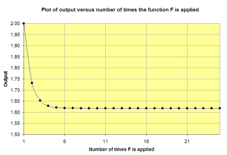
We see that after the $19^{th}$ iteration of the function $F$ the output does not change even in the $9^{th}$ decimal place.

A plot of the output versus the number of iterations of the function $F$ shows how rapidly the outputs approach the Â limiting value:

(Almost) any starting value will give the same result

If you experiment with different starting values, other than 3, you will see that repeatedly applying the function $F(x)=sqrt{1+x}$ to the output leads, after just a few iterations, to what seems to be the same decimal number.

An exception to this is if we choose a starting value less than -1, for example $x=-2$ . For then, we would have to take the square root of a negative number (and to do this we would have to use complex numbers, and get into all sorts of hot water about which value of the square root to take).

Cobwebs

When we carry out the iteration above we start with an input value, such as $x=3$ and get an output y-value $y=sqrt{1+3}=2$ .

We than use this output y-value as the new input x-value: $x= 2$ . This, in turn, produces a new output y-value: $y=sqrt{1+2}=sqrt{3}approx 1.732051$ .

We continue doing this – using the output y-value as the new input x-value -Â until the answer seems to stabilize.

There is a geometric way of seeing how this iteration process takes place, that helps us see how the output values stabilize.

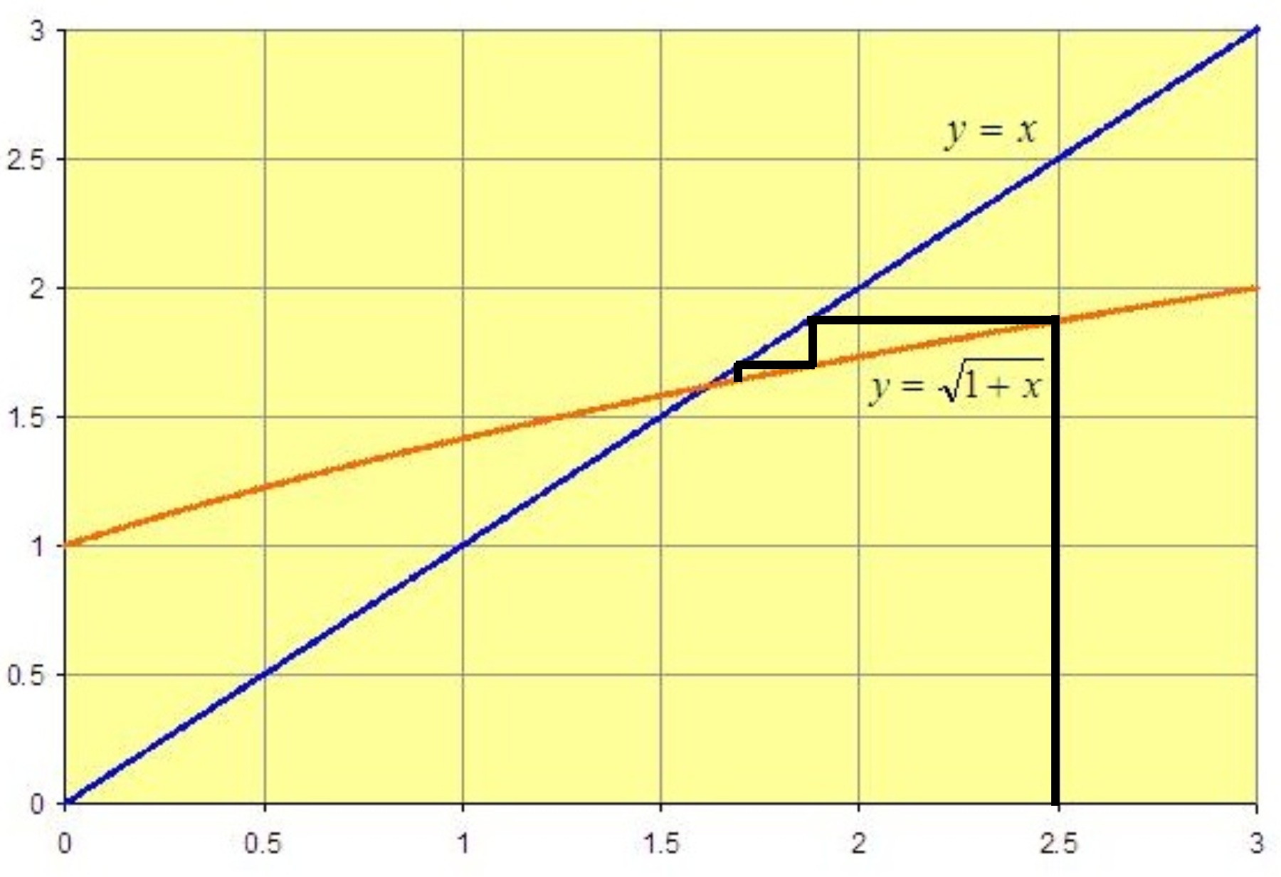
Suppose we start with the x-value $x=2.5$ .

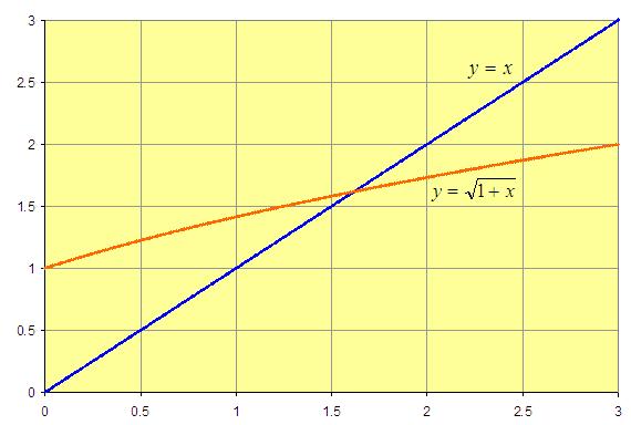
We draw the graphs of Â $y=sqrt{1+x}$ and $y=x$ :

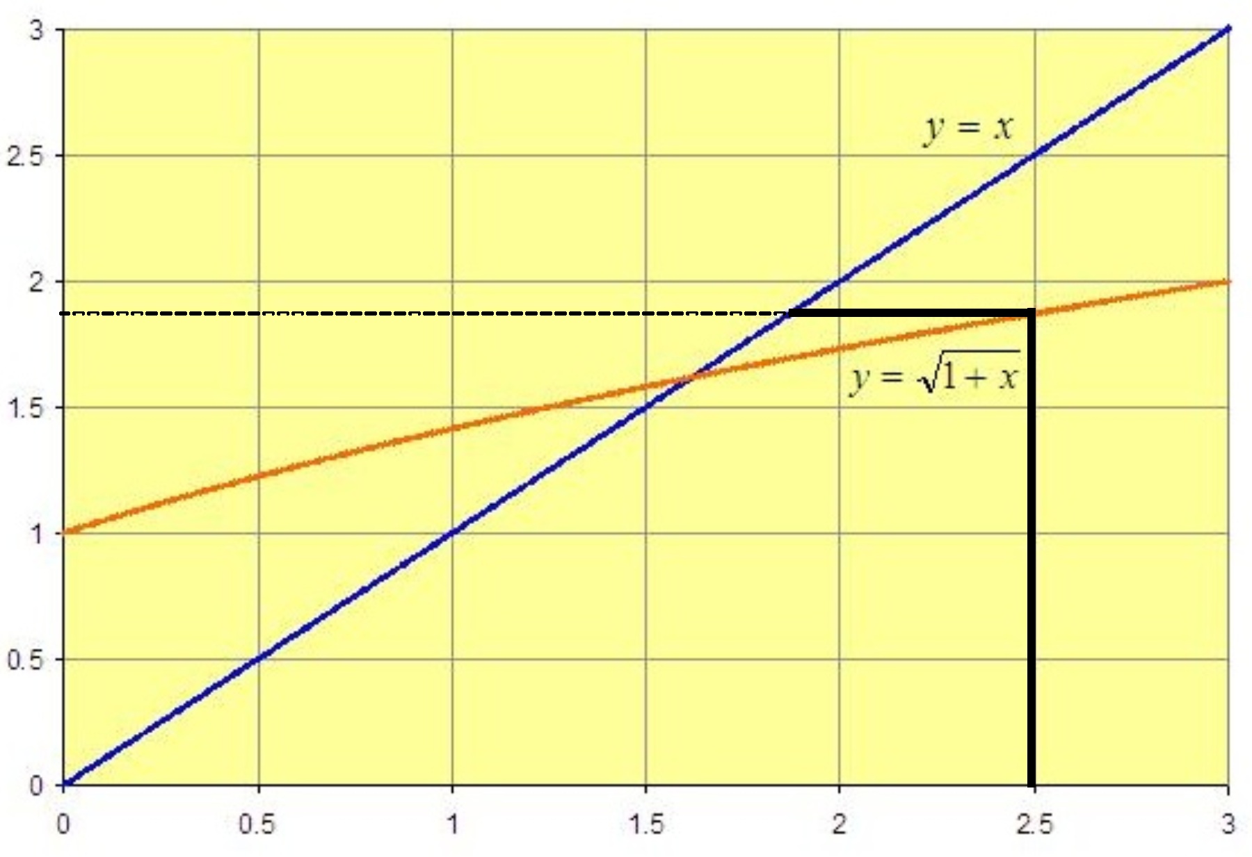
Geometrically, we find the output y-value by drawing a vertical line from the input x-value, $x=2.5$ , up until it meets the (orange) graph of $F(x)=sqrt{1+x}$ , and then drawing a horizontal line from that point to the vertical axis:

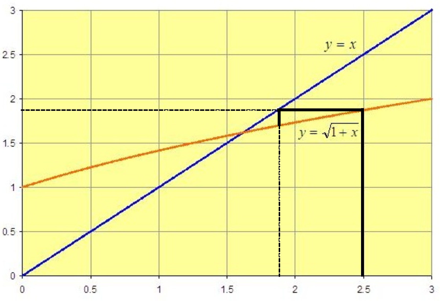
To take that output value as the input value we draw a horizontal line to the (blue) y=x line, and then drop a vertical line onto the x-axis:

By eliminating the repetitious drawing of lines to the y-axis and the x-axis we get the following cobweb diagram, which shows geometrically what the iterations of the function $F$ do to the starting point:

The iterates – the successive outputs – are converging rapidly to a number $phi$ where $F(phi)=phi$ . Using the formula for $F(x)$ we see that the iterates converge to the solution of $sqrt{1+x}=x$ . Because this point of convergence is positive, this condition is equivalent to $1+x=x^2$ which tells us that the point of convergence $x$ is the positive root of the quadratic equation:

$x^2-x-1=0$

The quadratic formula tells us that this is $phi=frac{1+sqrt{5}}{2} approx 1.618033989$ .

Continued fraction

Cleve mentions in his chapter on iteration that the equation for the fixed point $phi$ of the function $F$ also satisfies $phi= 1+frac{1}{phi}$ as one easily sees by dividing the quadratic expression for $phi$ by $phi$ .

This double mention of $phi$ on both sides of the expression $phi= 1+frac{1}{phi}$ allows us to write:

$phi=1+frac{1}{1+frac{1}{phi}}$

Applying that idea again we see that:

$phi=1+frac{1}{1+frac{1}{frac{1}{1+phi}}}$

This makes it look like we should be able to write $phi$ as an infinite continued fraction:

$x=1+frac{1}{1+frac{1}{frac{1}{1+ldots}}}$

It is actually relatively easy to see that the fractions we get by terminating this infinite continued fraction at different points do converge to the positive root of $x^2-x-1=0$ .

These first few fractions are, successively:

$1=frac{1}{1}$