Growth rates of simple integer recurrences
Posted by: Gary Ernest Davis on: June 5, 2012
The sequence of integers defined by
– where
, the floor of
, is the greatest integer
– begins 2, 3, 4, 6, 9, 13, 19, 28, 42, 63, 94, 141, 211, 316, 474, 711, 1066, 1599, 2398, 3597, 5395, 8092, 12138, 18207, 27310, 40965, 61447, 92170, 138255, 207382, 311073 and grows rapidly.
One can numerically estimate the growth rate of this sequence by first observing that the sequence of positive numbers is decreasing. This follows from the inequality
upon dividing by
, to get
.
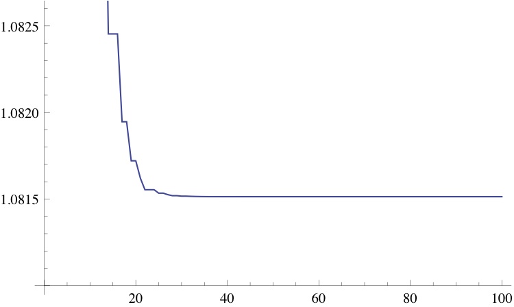
This means the sequence has a limit. In fact this sequence converges fairly rapidly to the limit:
| n | A(n)/(3/2)n | n | A(n)/(3/2)n | |
| 1 | 1.33333333333 | 34 | 1.08151439525 | |
| 2 | 1.33333333333 | 35 | 1.08151405187 | |
| 3 | 1.18518518519 | 36 | 1.08151382295 | |
| 4 | 1.18518518519 | 37 | 1.08151382295 | |
| 5 | 1.18518518519 | 38 | 1.08151382295 | |
| 6 | 1.14128943759 | 39 | 1.08151375512 | |
| 7 | 1.11202560585 | 40 | 1.08151375512 | |
| 8 | 1.09251638470 | 41 | 1.08151372497 | |
| 9 | 1.09251638470 | 42 | 1.08151370487 | |
| 10 | 1.09251638470 | 43 | 1.08151369148 | |
| 11 | 1.08673587473 | 44 | 1.08151368254 | |
| 12 | 1.08673587473 | 45 | 1.08151367659 | |
| 13 | 1.08416675918 | 46 | 1.08151367262 | |
| 14 | 1.08245401549 | 47 | 1.08151366997 | |
| 15 | 1.08245401549 | 48 | 1.08151366997 | |
| 16 | 1.08245401549 | 49 | 1.08151366880 | |
| 17 | 1.08194653587 | 50 | 1.08151366880 | |
| 18 | 1.08194653587 | 51 | 1.08151366880 | |
| 19 | 1.08172098938 | 52 | 1.08151366880 | |
| 20 | 1.08172098938 | 53 | 1.08151366880 | |
| 21 | 1.08162074649 | 54 | 1.08151366880 | |
| 22 | 1.08155391790 | 55 | 1.08151366869 | |
| 23 | 1.08155391790 | 56 | 1.08151366862 | |
| 24 | 1.08155391790 | 57 | 1.08151366862 | |
| 25 | 1.08153411684 | 58 | 1.08151366862 | |
| 26 | 1.08153411684 | 59 | 1.08151366860 | |
| 27 | 1.08152531636 | 60 | 1.08151366860 | |
| 28 | 1.08151944938 | 61 | 1.08151366859 | |
| 29 | 1.08151944938 | 62 | 1.08151366859 | |
| 30 | 1.08151684183 | 63 | 1.08151366859 | |
| 31 | 1.08151684183 | 64 | 1.08151366859 | |
| 32 | 1.08151568292 | 65 | 1.08151366859 | |
| 33 | 1.08151491032 | 66 | 1.08151366859 |
x
So we see that for large
.
What if we replace the constant 3/2 by a parameter ?
How does the sequence defined by
grow?
As before we see there is a constant such that
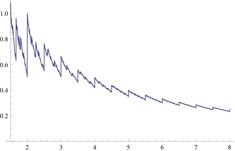
An obvious question is: how does ?
A moment’s thought shows that the answer is only interesting for
The following Mathematica® code computes to a decent approximation:
A[1, r_] = 2;
A[n_, r_] := A[n, r] = Floor[r*A[n – 1, r]];
T = Table[{r, Table[N[A[n, r]/r^n], {n, 1, 100}][[-1]]}, {r, 1.5, 5, 0.001}];
ListPlot[T, Joined -> True]
and the resulting plot of looks as follows:
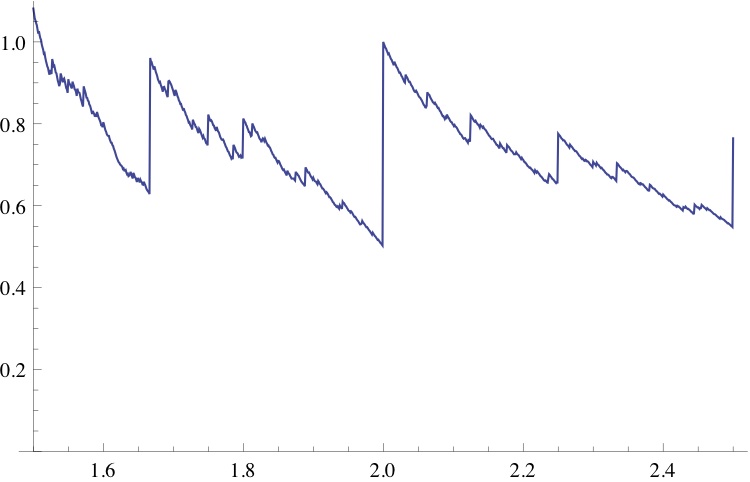
A blow-up of the portion of the plot for looks as follows:
Mississippi, West Virginia and Alabama biggest losers in obesity stakes – Colorado clear winner
Posted by: Gary Ernest Davis on: June 5, 2012
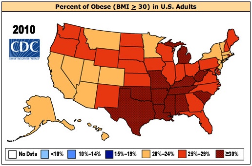
The Centers for Disease Control and Prevention website has a very interesting series of graphics depicting adult obesity rates in the United States by State and by year from 1985 through 2010.
Obesity for this purpose is defined as a body mass index (BMI) of 30 or above.
The changes year by year are dramatic.
The percentages of adults in the various states that are obese by this definition are shown for 2010 in the graphic below:
The States, buy sorted by percentage of obese adults from largest to smallest, patient is shown in the table below, together i the z-scores for those percentages (for this purpose the District of Columbia is counted as a State)
| STATE | % PEOPLE WITH BMI >30 | Z-SCORE |
| Mississippi | 34 | 2.17 |
| West Virginia | 32.5 | 1.70 |
| Alabama | 32.2 | 1.61 |
| South Carolina | 31.5 | 1.40 |
| Kentucky | 31.3 | 1.33 |
| Texas | 31 | 1.24 |
| Louisiana | 31 | 1.24 |
| Michigan | 30.9 | 1.21 |
| Tennessee | 30.8 | 1.18 |
| Missouri | 30.5 | 1.09 |
| Oklahoma | 30.4 | 1.05 |
| Arkansas | 30.1 | 0.96 |
| Indiana | 29.6 | 0.81 |
| Georgia | 29.6 | 0.81 |
| Kansas | 29.4 | 0.75 |
| Ohio | 29.2 | 0.68 |
| Pennsylvania | 28.6 | 0.50 |
| Iowa | 28.4 | 0.44 |
| Illinois | 28.2 | 0.37 |
| Delaware | 28 | 0.31 |
| North Carolina | 27.8 | 0.25 |
| South Dakota | 27.3 | 0.10 |
| North Dakota | 27.2 | 0.06 |
| Maryland | 27.1 | 0.03 |
| Nebraska | 26.9 | -0.03 |
| Maine | 26.8 | -0.06 |
| Oregon | 26.8 | -0.06 |
| Florida | 26.6 | -0.12 |
| Idaho | 26.5 | -0.15 |
| Wisconsin | 26.3 | -0.21 |
| Virginia | 26 | -0.31 |
| Rhode Island | 25.5 | -0.46 |
| Washington | 25.5 | -0.46 |
| New Mexico | 25.1 | -0.58 |
| Wyoming | 25.1 | -0.58 |
| New Hampshire | 25 | -0.62 |
| Minnesota | 24.8 | -0.68 |
| Alaska | 24.5 | -0.77 |
| Arizona | 24.3 | -0.83 |
| California | 24 | -0.92 |
| New York | 23.9 | -0.96 |
| New Jersey | 23.8 | -0.99 |
| Vermont | 23.2 | -1.17 |
| Montana | 23 | -1.23 |
| Massachusetts | 23 | -1.23 |
| Hawaii | 22.7 | -1.33 |
| Utah | 22.5 | -1.39 |
| Connecticut | 22.5 | -1.39 |
| Nevada | 22.4 | -1.42 |
| District of Columbia | 22.2 | -1.48 |
| Colorado | 21 | -1.85 |
x
The States with a z-score greater than 1 are Mississippi, West Virginia, Alabama, South Carolina, Kentucky, Texas, Louisiana, Michigan, Tennessee, Missouri and Oklahoma.
The States with a z-score less than -1 are Vermont, Montana, Massachusetts, Hawaii, Utah, Connecticut, Nevada,District of Columbia and Colorado.
Mississippi is at the extreme with a z-score above 2, and Colorado lies at the other extreme with a z-score of almost -2
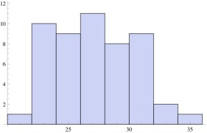
These outliers can be visualized from the histogram of the percentages of obese adults:
This histogram is fairly flat, indicating a relatively uniform distribution with the exception of Colorado, with only 21% of obese adults, at the low end, Â and Alabama, West Virginia and Mississippi with more than 32% of obese adults, at the high end.
Southern cooking might be tasty, but it seems there might be something about the mountain air of Colorado that is associated with a lower obesity rate.
On the other hand, if we multiply the percentage rates of obese adults by the population, for each state, we get the number of obese adults per state:
| STATE | OBESE POPULATION/ 2010 | Z-SCORE |
| Â California |
8940949 |
4.04 |
| Â Texas |
7795124 |
3.41 |
| Â Florida |
5001148 |
1.86 |
| Â New York |
4631366 |
1.65 |
| Â Pennsylvania |
3632880 |
1.10 |
| Â Illinois |
3618238 |
1.09 |
| Â Ohio |
3368659 |
0.95 |
| Â Michigan |
3054045 |
0.78 |
| Â Georgia |
2867545 |
0.68 |
| Â North Carolina |
2650864 |
0.56 |
| Â New Jersey |
2092471 |
0.25 |
| Â Virginia |
2080266 |
0.24 |
| Â Tennessee |
1954600 |
0.17 |
| Â Indiana |
1919205 |
0.15 |
| Â Missouri |
1826623 |
0.10 |
| Â Washington |
1714758 |
0.04 |
| Â Maryland |
1564633 |
-0.05 |
| Â Arizona |
1553260 |
-0.05 |
| Â Alabama |
1539075 |
-0.06 |
| Â Massachusetts |
1505955 |
-0.08 |
| Â Wisconsin |
1495677 |
-0.08 |
| Â South Carolina |
1456990 |
-0.10 |
| Â Louisiana |
1405345 |
-0.13 |
| Â Kentucky |
1358222 |
-0.16 |
| Â Minnesota |
1315373 |
-0.18 |
| Â Oklahoma |
1140411 |
-0.28 |
| Â Colorado |
1056131 |
-0.33 |
| Â Oregon |
1026728 |
-0.34 |
| Â Mississippi |
1008881 |
-0.35 |
| Â Arkansas |
877691 |
-0.43 |
| Â Iowa |
865165 |
-0.43 |
| Â Kansas |
838817 |
-0.45 |
| Â Connecticut |
804172 |
-0.47 |
| Â Utah |
621874 |
-0.57 |
| Â Nevada |
604923 |
-0.58 |
| Â West Virginia |
602223 |
-0.58 |
| Â New Mexico |
516854 |
-0.63 |
| Â Nebraska |
491286 |
-0.64 |
| Â Idaho |
415409 |
-0.68 |
| Â Maine |
356001 |
-0.71 |
| Â New Hampshire |
329118 |
-0.73 |
| Â Hawaii |
308788 |
-0.74 |
| Â Rhode Island |
268405 |
-0.76 |
| Â Delaware |
251422 |
-0.77 |
| Â Montana |
227565 |
-0.79 |
| Â South Dakota |
222271 |
-0.79 |
| Â North Dakota |
182945 |
-0.81 |
| Â Alaska |
174007 |
-0.82 |
| Â Vermont |
145172 |
-0.83 |
| Â Wyoming |
141470 |
-0.83 |
| Â Washington, DC |
133583 |
-0.84 |
We see that California and Texas account for a significant number of the total of obese adults in the US.
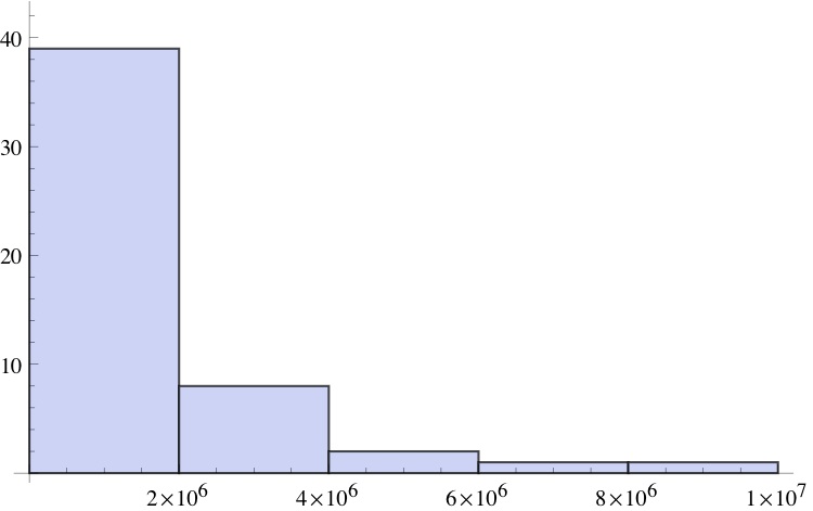
A histogram of the population data for obesity shows how skewed is the distribution of state numbers of obese adults (as distinct from percentages)Â :
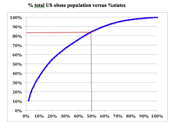
In fact, if we plot the cumulative percentage of obese adults in the states, versus the cumulative percentage (out of 51) of the states (including DC) we get the following curve, which shows, for example, that the half the states account for approximately 85% of all US obese adults:
