Republic of Mathematics blog

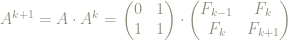
Some fun with a (very) simple matrix

Posted by: Gary Ernest Davis on: February 20, 2011

In: Uncategorized
Leave a Comment

Geometry of a transformation

The $2\times 2$ matrix $A=\begin{pmatrix} 0 & 1 \\1 & 1 \end{pmatrix}$ is very simple: it has entries consisting only of 0’s and 1’s.

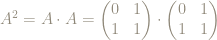
As a $2\times 2$ matrix we can think of $A$ as transforming points in the euclidean plane. These are points with coordinates $(x,y)$ where $x \textrm{ and } y$ are real numbers.

The matrix $A$ transforms the point $(x,y)$ into the point $A\cdot (x,y) = \begin{pmatrix} 0 & 1 \\1 & 1 \end{pmatrix}\cdot (x,y):= (y, x+y)$ :

We can look at what the matrix $A$ does to geometric shapes in the plane.

For example, the square with corners $(0,0), (1,0), (0,1), (1,1)$ – show in yellow in the diagram below – gets transformed into the parallelogram with corners $(0,0), (0,1), (1,1), (1,2)$ – shown in purple dots in the diagram below:

The area of the parallelogram is 1 unit – the same as the area of the original square. Because area of any plane figure is based on counting squares – and taking a limit with vanishingly small squares if the figure is somewhat round, such as a circular region – the matrix $A$ is an area-preserving transformation of the plane.

However if we imagine traveling counter-clockwise from the point $(1,0)$ to the point $(0,1)$ we see that the transformation $A$ has us traveling clockwise from $A\cdot(1,0) = (0,1)$ to $A\cdot(0,1) = (1,1)$ :

In other words, the matrix $A$ is an orientation-reversing transformation of the plane.

Appearance of the Fibonacci numbers

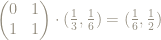
What happens when we apply the matrix over and over to a point?

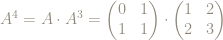
For instance, if we apply the matrix $A$ to the point $(x,y)$ Â we get the point $A\cdot (x,y)=(y,x+y)$ , and if we then apply $A$ to this new point we get the point $A\cdot (y,x+y) =(x+y,x+2y)$ .

This is the same result as if we had applied the square $A^2=\begin{pmatrix} 0 & 1 \\1 & 1 \end{pmatrix}\cdot \begin{pmatrix} 0 & 1 \\1 & 1 \end{pmatrix} =\begin{pmatrix} 1 & 1 \\1 & 2 \end{pmatrix}$ to the point $(x,y)$ .

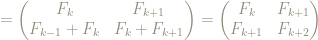
This is true more generally: to figure out what applying the matrix $A$ over and over does to a point $(x,y)$ , it is the same as working out the appropriate power of the matrix $A$ and applying that matrix to $(x,y)$ .

So can we characterize, or identify, the powers of the matrix $A=\begin{pmatrix} 0 & 1 \\1 & 1 \end{pmatrix}$ ?

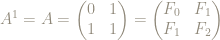
Here are the first few powers:

$A^1=\begin{pmatrix} 0 & 1 \\1 & 1 \end{pmatrix}$

$A^2=A\cdot A=\begin{pmatrix} 0 & 1 \\1 & 1 \end{pmatrix}\cdot \begin{pmatrix} 0 & 1 \\1 & 1 \end{pmatrix}$

$=\begin{pmatrix} 1 & 1 \\1 & 2 \end{pmatrix}$

$A^3=A\cdot A^2=\begin{pmatrix} 0 & 1 \\1 & 1 \end{pmatrix}\cdot \begin{pmatrix} 1 & 1 \\1 & 2 \end{pmatrix}$

$= \begin{pmatrix} 1 & 2 \\2 & 3 \end{pmatrix}$

$A^4=A\cdot A^3=\begin{pmatrix} 0 & 1 \\1 & 1 \end{pmatrix}\cdot \begin{pmatrix} 1 & 2 \\2 & 3 \end{pmatrix}$

$= \begin{pmatrix} 2 & 3 \\3 & 5 \end{pmatrix}$

$A^5=A\cdot A^4=\begin{pmatrix} 0 & 1 \\1 & 1 \end{pmatrix}\cdot \begin{pmatrix} 2 & 3 \\3 & 5 \end{pmatrix}$

$= \begin{pmatrix} 3 & 5 \\5 & 8 \end{pmatrix}$

These matrix entries are looking suspiciously familiar: they are looking like the Fibonacci numbers $1, 2, 3, 5, 8, \ldots$

Have we just been lucky so far, or is this something we can prove?

A good proof technique for this sort of problem is proof by induction, because we know inductively how to work out the powers ofÂ the matrix $A$ , namely $A^1=A \textrm{ and } A^{n+1}=A\cdot A^n$ .

First, we need a precise statement of what it is we are trying to prove.

It’s looking like:

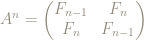
$A^n= \begin{pmatrix} F_{n-1} & F_n \\F_n & F_{n-1} \end{pmatrix}$ where $F_n$ are the Fibonacci numbers given by $F_0=0, F_1=1, F_n=F_{n-1}+F_{n-2}\textrm{ for } n\geq 2$ , namely $0, 1, 1, 2, 3, 5, 8, \ldots$

This is certainly true for $n=1$ because $A^1=A=\begin{pmatrix} 0 & 1 \\1 & 1 \end{pmatrix}=\begin{pmatrix} F_0 & F_1 \\F_1 & F_2 \end{pmatrix}$

So let’s suppose that it’s true for some particular value of $n$ , say $n=k$ (for example: $k=1$ ).

Then $A^{k+1}=A\cdot A^k = \begin{pmatrix} 0 & 1 \\1 & 1 \end{pmatrix}\cdot \begin{pmatrix} F_{k-1} & F_k \\F_k & F_{k+1} \end{pmatrix}$

$=\begin{pmatrix} F_k & F_{k+1} \\F_{k-1}+F_k & F_k+F_{k+1} \end{pmatrix}=\begin{pmatrix} F_k & F_{k+1} \\F_{k+1} & F_{k+2} \end{pmatrix}$

so our statement is true also for $n=k+1$ . By the principle of mathematical induction, it is true for all $n\geq 1$ .

Moving to a torus

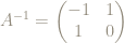
The matrix 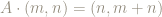$A$ has the property that it sends points in the plane with integer coordinates to similar points: $A\cdot (m,n)=(n,m+n)$ so if $m, n$ are integers then so are the coordinates of $A\cdot (m,n)$ .

This means we can restrict $A$ as a transformation of the unit square with corners $(0,0), (1,0), (0,1), (1,1)$ so long as we keep only the fractional parts of the coordinates of points.

For example, the point $(\frac{3}{4},\frac{2}{3})$ lies in the unit square but it’s transformation by the matrix $A$ does not: $A\cdot (\frac{3}{4},\frac{2}{3}) = (\frac{2}{3},\frac{17}{12})$ . So we reduce the result by keeping only the fractional parts of the coordinates: $(\frac{2}{3},\frac{5}{12})$ .

This operation, of reducing coordinates by keeping only the fractional parts is called reduction modulo 1.

Wwe write the result of keeping only the fractional parts of the coordinates of the point $(x,y)$ as $(x,y) \textrm{ mod }1$

When we think about this for a moment we see that some apparently different points on the unit square are actually the same, modulo 1.

For example, any point of the form $(t,0) \textrm{ where } 0\leq t\leq 1$ is the same, modulo 1, as the point $(t,1)$ .

Ditto, any point 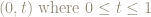$(0,t) \textrm{ where } 0\leq t\leq 1$ is the same, modulo 1, as the point $(1,t)$ .

This means the sides of the squares, are really the same line, modulo 1:

We can get a different picture of the unit square, modulo 1,Â if we glue together points on the square that are the same modulo 1.

First we can glue corresponding points on the blue sides to get a cylinder:

Now, when we glue together the red ends of the cylinder, as indicated, we get the surface of a donut, otherwise known as a torus:

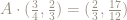
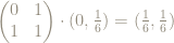
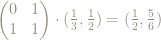
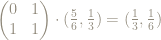
So now we can use the matrix $A$ to transform points on the torus, so long as we remember to reduce the coordinates of the points modulo 1.

What happens if, for example, we begin with the point $(\frac{1}{2},\frac{1}{3})$ and keep applying the matrix $A$ over to the result?

$\begin{pmatrix} 0 & 1 \\1 & 1 \end{pmatrix}\cdot (\frac{1}{2},\frac{1}{3})=(\frac{1}{3},\frac{5}{6})$

$\begin{pmatrix} 0 & 1 \\1 & 1 \end{pmatrix}\cdot (\frac{1}{3},\frac{5}{6})=(\frac{5}{6},\frac{1}{6})$ (remember we are reducing modulo 1)

$\begin{pmatrix} 0 & 1 \\1 & 1 \end{pmatrix}\cdot (\frac{5}{5},{1}{6})=(\frac{1}{6},0)$

$\begin{pmatrix} 0 & 1 \\1 & 1 \end{pmatrix}\cdot (\frac{1}{6},0)=(0,\frac{1}{6})$

$\begin{pmatrix} 0 & 1 \\1 & 1 \end{pmatrix}\cdot (0,\frac{1}{6})=(\frac{1}{6},\frac{1}{6})$

$\begin{pmatrix} 0 & 1 \\1 & 1 \end{pmatrix}\cdot (\frac{1}{6},\frac{1}{6})=(\frac{1}{6},\frac{1}{3})$

$\begin{pmatrix} 0 & 1 \\1 & 1 \end{pmatrix}\cdot (\frac{1}{6},\frac{1}{3})=(\frac{1}{3},\frac{1}{2})$

$\begin{pmatrix} 0 & 1 \\1 & 1 \end{pmatrix}\cdot (\frac{1}{3},\frac{1}{2})=(\frac{1}{2},\frac{5}{6})$

$\begin{pmatrix} 0 & 1 \\1 & 1 \end{pmatrix}\cdot (\frac{1}{2},\frac{5}{6})=(\frac{5}{6},\frac{1}{3})$

$\begin{pmatrix} 0 & 1 \\1 & 1 \end{pmatrix}\cdot (\frac{5}{6},\frac{1}{3})=(\frac{1}{3},\frac{1}{6})$

$\begin{pmatrix} 0 & 1 \\1 & 1 \end{pmatrix}\cdot (\frac{1}{3},\frac{1}{6})=(\frac{1}{6},\frac{1}{2})$

$\begin{pmatrix} 0 & 1 \\1 & 1 \end{pmatrix}\cdot (\frac{1}{6},\frac{1}{2})=(\frac{1}{2},\frac{1}{3})$

and we are back to where we started, after 13 steps.

The collection 12 points we collected along the way: $(\frac{1}{3},\frac{5}{6}), (\frac{5}{6},\frac{1}{6}), \ldots$ is called the orbit of the initial point $(\frac{1}{3},\frac{5}{6})$ .

Any of the points in the orbit of $(\frac{1}{3},\frac{5}{6})$ has exactly the same 12 points as its orbit. This is because the matrix $A$ is an invertible matrix with inverse $A^{-1}=\begin{pmatrix} -1 & 1 \\1 & 0 \end{pmatrix}$

Just as for the point we chose, any point on the torus with rational number coordinates will have a finite orbit.

Question 1: Can you see why this is so?

Question 2: Can you figure out the size of the orbit of the point $(\frac{a}{b},\frac{c}{d})$ from the numbers $a, b, c, d$ ?

Wherever we are on the torus there is a point nearby – as close as we wish – that has rational coordinates. Therefore, wherever we are on the torus there is a point nearby – as close as we wish – with a finite orbit.

Arnold’s cat map

The square of the matrix $A$ , namely the matrix $\begin{pmatrix} 1 & 1 \\1 & 2 \end{pmatrix}$ is known as Arnold’s cat map.

This matrix gives us an area-preserving, orientation-preserving transformation of the torus, that like the matrix $A$ is technically chaotic.

What this means in practice is that when we take two points on the torus that are very close together, and examine points in their orbit we will soon find corresponding points that are quite far apart.

Then as we progress through the orbits we will find the points get back close together again.

Vladimir Arnold

Vladimir Arnold visualized this by imagining a picture of a cat drawn on the torus and seeing what happened to the cat as we repeatedly applied the matrix transformation .

The cat would at first get spread all over the torus but would eventually become almost reconstructed.

A lovely account of Arnold’s cat map appears in the articleÂ “Period of a discrete cat mapping” by Freeman Dyson and Harold Falk.

Tags: Arnold, cat map, Fibonacci, Freeman Dyson, math, mathematics, ttransformation

First steps in differential equations: learning to see and to think

Posted by: Gary Ernest Davis on: February 19, 2011

In: Uncategorized
2 Comments

Differential equations and studio learning

This semester I am once again teaching introductory differential equations.

The students in this class are mainly engineering majors, with some mathematics and physics majors, for whom the course is mandatory. Occasionally a humanities or business major will enroll in this class for interest, but not this semester.

The computer laboratory where the class meets has 16 computers, each shared by two students, so the maximum class enrollment is 32.Â Of those 32 most are young – usually sophomore – males, but this semester there are 6 females: 5 engineering majors and 1 mathematics major.

I run this course as a studio class in which students have projects to work on in pairs. Projects last from 2-3 weeks, and all work in progress and final reports must be placed on WordPress blogs. A class list with active links to individual student blogs allows all students to readily see all other student work.

After completion of a project I write critiques on individual student blogs, together with a putative grade for each student. Students may revise earlier projects and ask me to regrade them (If, however, they submit nothing by the due date they receive zero for that project).

Students are advised in writing, and in periodic class announcements, of the University policy on plagiarism, and of the need to make all written work their own. Naturally, students who work for 6 or so classes at the same computer, doing and discussing the same calculations, will have a lot in common to write about. They must, however, tell their own story in their own words. This also means avoiding lengthy quotes from other students, in lieu of writing their own thoughts and conclusions.
I was experimenting with this approach to teaching and learning some time before I came across John Seely Brown’s excellent account of the effects of studio-style teaching on student learning:

Learning to see

The first thing I have the students do is plot vector fields of differential equations and to examine those plots for characteristic features.

I use Mathematica for this purpose because it is more widely available in the Universty than MATLAB or Maple, and also, in my view, produces better graphics (that, of course, is an arguable point). Mathematica has a streamplot option which draws candidate integral curves of a differential equations, and so allows a student to be able to better see what potential solution curves look like.

This, to my mind, is somewhat like looking at paintings in an art history course – learning to see more deeply.

Here’s a couple of examples where the students have some difficulty putting what they think they see into words:

$\frac{dy}{dx}=\frac{x-y}{x+y}$

$\frac{dy}{dx}=-\frac{2xy}{x^2+y^2}$

A couple of students discussed what appear to be hyperbolic forms in the first example, and quite a few more discussed the appearance of asymptotes. Many more, however, described the plot as being composed of a bunch or parabolas.

We can imagine what’s going on in their minds here: they are clutching at words that sound appropriate, words such as “parabola” for something generally curved.

The first thing I wanted them to do, however, was to look into the plot and tell me what they saw.

Of course, looking is not just an act of having light hit one’s eyeballs: it is an active process of interpreting what is in front of one’s eyes, and an active process of seeking out finer, previously unnoticed, details. It is, in other words, an intelligent process.

This, is quite unlike anything these students have encountered before in a mathematics class.

Previous mathematics classes have been about doing calculations, solving problems, or trying to construct proofs.

No one in their prior experience has asked them to look at a relatively complicated mathematical plot andÂ describe in depth and detail what they saw.

But, of course, if vector plots of differential equations are to be useful to the practicing engineer, mathematician and scientist (and they are) then those professionals must be able to look deeply and interpret what the machine has produced.

The striking symmetry in the second plot was mentioned by only one student, and then not fully. Only one student mentioned that the solution curves approach 0 at $\pm\infty$ and reach a maximum (or minimum, respectively) at $x=0$ .

There was a lot going on in these first two weeks that students had to get used to: working in pairs with other students they did not know, learning to use WordPress and write LaTeX, and learning to use Mathematica, and get the graphics output in jpeg format t o upload to WordPress.

It’s understandable they thought the main task was to get something done, and that something was to produce nice vector plots.

It’s taking them some time to understand that my main focus is on looking deeply into what the plots tell us.

Learning to think

Only one of the 32 students attempted to predict, from the form of a differential equation, what the solution curves might look like:

$\frac{dy}{dx}=\frac{x-y}{x+y}$

“So if you look at this function analytically I suppose any time x=y the function equals zero because the argument in the numerator is (x-y) and subtracting equal values gives you zero. In the denominator I would expect an asymptote if y=-x because summing them would create a zero in the denominator and making the function undefined.”

To be fair, I did not say in writing that students should relate features of the differential equation to likely solution curves, or having seen the streamline plot, say what aspects of the solution curves correspond to what features of the differential equations. But I did say this verbally in class on several occasions, and did talk about it in depth with several groups of students.

Overall, I am not unhappy. The students are moving more slowly than I hoped for and would like. But they have got things working, and even though there is another topic and project now well under way, they have a chance to go back and to take time to look again at their plots and see how features of the differential equation are reflected in features of the plots.

They have a chance, in other words, to look, to see, to think, and to learn.

Can this really be mathematics? they ask.

Tags: differential equations, mathematics, Teaching 2.0