Republic of Mathematics blog

Robo-math

Will it soon come to this?

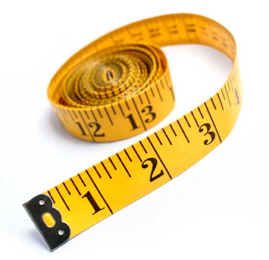
For several years,  I attempted to  teach pre-service teachers about the normal distribution through the distribution of measurement “errors”. I would find a male student who was willing to have his chest measured and ask other students in the class to take turns measuring his chest as accurately as possible – to the nearest of an inch.

Students, of course, tried to be very accurate.

I, of course, knew that such repeated fine measurement of such a large object as a chest was going to produce a distribution of values. My plan was to get the students to show the differences around the average of their measurements.

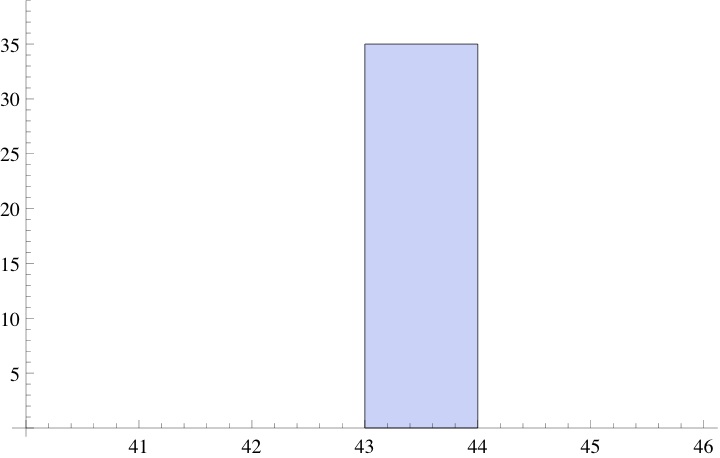
If I had asked the students to measure to the nearest inch, a histogram of their measurements would most likely have produced something like the following:

Asking them to measure to the nearest inch  a chest that’s around 43″ pretty much guarantees very little variance: most, if not all, students will record a measurement of 43″.

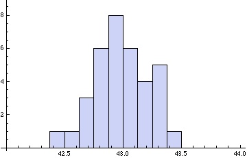
If, however, they have to measure to the nearest of an inch a lot of variation will creep in. This variation is due to slips in the measuring tape, slips in reading the answer accurately, slight changes in the chest due to breathing, slightly different measurement places – higher or low on the chest. In other words, many tiny factors will operate to produce considerable variation in the students’ recorded measurements.

A histogram of their measurements will now look more like this:

Students will often ask at this point: “but what is the true measurement?”

My answer is that repeated measurement does not produce a number – it produces a distribution of numbers. The answer to the question: “How large is this man’s chest?” is not a number: it is a distribution. This distribution reflects the process of repeated measurement.

Reliability

It’s sort of obvious that if we use a relatively large measurement unit – such as 1″ to measure a 43″ chest, – several people’s independent  measurements will give a very reliable result: pretty much 43″ every time. What is equally obvious is that as we decrease the unit of measurement – down, say, to of an inch – various factors come into play to make our measurements less reliable. The more spread the measurements distribution is from the average, the less reliable is the measurement process.

A single measurement returns a number. A series of independent measurements – which is at the basis of scientific replicability – returns a distribution of numbers, more or less spread out around the average.

The “true” measure

Just as students often ask what is the correct value for the chest measurement, so science, in its application of statistics, assumes there is a number that is the true measure, and that our measurement process is an attempt to estimate that true value. This is a hypothesis at best, and does not genuinely reflect the human nature of, and involvement in, measurement. Who has access to this “true” measurement is a mystery to me. The more accurately we try to measure, the more likely we are to obtain a spread-out distribution of measurements.

Every set of independent measurements will produce a distribution of numerical values and that distribution, like all other distributions, has certain descriptive properties such as central measures, measures of variation, measures of symmetry, and of peakedness (otherwise known as kurtosis).

The true score theory, or true measurement theory, postulates (and it is only a postulate) that a measurement value is the sum of a true value and a possibly random error : .

This postulate has an interesting consequence that I have rarely seen discussed. Suppose, as was the case in our pre-service teacher’s measurement process that measurements were carried out in a sequence, one following the other. This means – assuming a class size of – that we had a sequence of measurements . The true score, or true measurement, theory postulates that each . The so-called “error” terms can be thought of as random variables. Now we see that

The terms are random variables, so if they are identically distributed, as one might reasonably imagine, we can view the measurement as being obtained from the initial measurement by a random walk: successive measurements in a sequence of independent measurements are random excursions from a previous measurement.

“So what?” you may ask.

Well, the above consequence of true score, or true measurement, theory does not mention the hypothesized “true value” .

In other words, this consequence of true measurement theory, does not mention “true value” and sees repeated measurements as a random walk.

This “random walk theory” of measurement – for want of a better phrase – compels us to focus right from the beginning on the statistical aspects of measurement, rather then being side-tracked by a hypothetical “true value”.

Form this perspective, repeated measurements are a random walk, specified statistically by the nature of the “error” distribution.

That the “errors” generally follow a normal distribution is another, and deeper, story.