Republic of Mathematics blog

Some peculiarities of higher dimensional spaces

Posted by: Gary Ernest Davis on: July 30, 2010

In: Uncategorized
2 Comments

These days, higher dimensional spaces are not regarded as weirdly as they were formerly. Most people – in the United States, at least – have seen the e-Harmony advertisements in which the company boasts it “matches single women and men based on 29 DimensionsÂ® of Compatibility“. And most educated people are more or less familiar with the idea of a 4-dimensional space-time continuum.

What is well-known to people working in optimization and in statistics, but less well-known generally, is that some of our intuitions about distribution of points do not serve us well in going from 2 and 3 dimensions to higher dimensions.

In this post I want to look at just one peculiar feature of the distribution of points in higher-dimensional space: the fact that in balls in higher dimensional space overwhelmingly most points lie close to the boundary of the ball.

We can see the beginnings of this peculiar distribution of points even in 2 dimensions, where fully 36% of a 10′ pizza with a 1″ crust lies on the crust. In higher dimensions this apparently uneven distribution of points becomes much more marked.

To begin our exploration of this phenomenon in higher dimensions we turn to Dave Richeson’s excellent account of the volumes of balls in higher dimensional spaces.

d-dimensional space Â consists of “points” $(x_1,\ldots x_d)$ where the $x_i$ are real numbers. Here are a few points in 5-dimensional space, generated randomly using MathematicaÂ®:

$p_1 = (18.4358, -12.4551, -14.42, 9.22485, -9.87961)$

$p_2 = (7.71709, 10.077, 11.4523, 15.0892, -18.0596)$

$p_3 = (-19.9767, 8.98969, -7.51896, 10.6999, -8.35938)$

The ball of radius $R>0$ in d-dimensional space consists of all points $(x_1,\ldots x_d)$ for which $\sqrt{x_i^2+\ldots x_d^2} \leq R$ .

The surface, or boundary, of the ball of radius R in d-dimensional space is the (d-1)-dimensional sphere, consisting of all points Â $(x_1,\ldots x_d)$ Â for which $\sqrt{x_i^2+\ldots x_d^2} = R$ .

I want to address the question: in a d-dimensional ball of radius R, what percentage of the volume of the ball is occupied by points lying within 10% of the boundary?

Fortunately the beautiful formula for the volume of a d-dimensional ball of radius R allows us to answer this question very easily: the volume of a d-dimensional ball of radius R is $\frac{\pi^{d/2}R^d}{\Gamma(d/2+1)}$ , where the gamma function $\Gamma(d/2+1) = \int_0^\infty t^{d/2}e^{-t}dt$ is a generalization of the factorial function to fractional values of the variable.

From this lovely formula we can easily calculate the ratio of the volume in the outermost 10% of the d-dimensional ball of radius R to the whole volume of this ball.

The volume in the outermost 10% is $\frac{\pi^{d/2}R^d}{\Gamma(d/2+1)}-\frac{\pi^{d/2}(0.9\times R)^d}{\Gamma(d/2+1)}$ .

The ratio of this to the volume of the entire ball is, after some simple algebra, $1-\frac{(0.9 \times R)^d}{R^d} = 1-0.9^d$ .

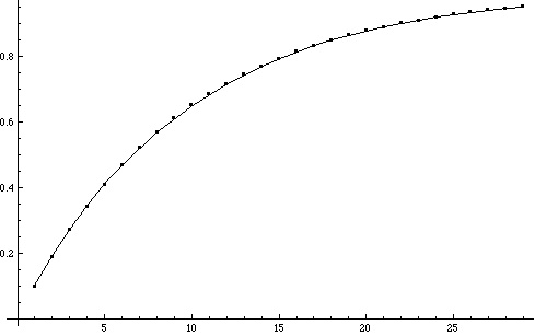
This quantity approaches 1 very rapidly as d increases:

By the time we reach 29-dimensional space, the percentage of volume of a 29-dimensional ball occupied by the 10% of the points nearest the boundary is a whopping 95.3%.

To put it slightly differently, a 29-dimensional ball of radius 0.9, has only 4.7% of the volume of a 29-dimensional ball of radius 1.

To put it in another graphic way, if we Â populate a 29-dimensional ball of radius R with a bunch of uniformly distributed points – that is, each small volume elements in the ball gets approximately the same number of points – then 95.3% of the points will lie within 10% of the boundary of the ball. Doesn’t this sound counter-intuitive? If the points are uniformly distributed in the ball shouldn’t just 10% of them lie within 10% of the boundary? The key thing to observe is that uniform distribution means each very small volume element gets about the right proportion of points, and the counter-intuitive fact that most of the volume of the ball lies near the boundary in high dimensional space.

How does this look in dimensions 2 and 3 where we can see the points in a ball?

To answer this question we first have to figure out how to choose a bunch of points randomly and uniformly in a ball. Â Fortunately this was resolved by George Marsaglia in 1972 who showed how to choose points uniformly on a sphere in d-dimensional space. 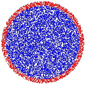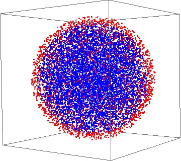First one chooses many points $v=(x_1,\ldots x_d)$ where the $x_i$ are normally distributed,Â and then divides each $v$ by its length $\Vert v \Vert$ ; we then choose uniformly random numbers $u$ between 0 and R, and multiply to get points $u\frac{v}{\Vert v \Vert}$ which are Â uniformly distributed in d-dimensional ball. Â This procedure is easily implemented in Mathematica, and here is the result of producing 10,000 points uniformly distributed in a 2-dimensional ball, and a 3-dimensional ball, respectively. The points within 10% of the boundary are colored red, and the other points blue:

10,000 points uniformly distributed in a 2-dimensional ball. 81.45% of the points are less than 0.9 from origin (blue), and 18.55% of the points greater than 0.9 from origin (red)

10,000 points uniformly distributed in a 3-dimensional ball. 73.99% of the points lie within 0.9 from origin (blue), and 26.01% of the points are greater than 0.9 from origin (red)

Addendum

Beginning August 2, 2010, Case Western Reserve University will host a conference “Perspectives in High Dimensions” dealing with asymptotic geometric analysis. V. D. Milman (2007) has written an Â overview of asymptotic geometric analysis: Asymptotic_geometric_analysis_ Milman

Computational media: the universal acid of mathematics teaching (6)

Posted by: Gary Ernest Davis on: April 28, 2010

In: Uncategorized
Leave a Comment

Computational media and “What if?”

Digital technology allows greater computational power in smaller and more portable, and affordable devices. Â By “computational” I do not mean only “doing sums”. Software such as Geogebra , Geometer’s Sketchpad and Cabri are also computational media. What makes them so is their use of computation to keep track of relationships between objects. These objects can be numbers, algebraic symbols or geometric points or constructions. Â Most computational media, from spreadsheets up, is dynamic. What this means is that the initial data or parameters can be updated and the medium automatically updates the established relationships between objects. Just as for spreadsheets, computational media begs us to ask the fundamental question “What if?”

What if we add two whole numbers? How will the oddness or evenness (parity) of the answer depend on that of each number? What if we multiply?
What if the coefficients of a quadratic function are chosen randomly? How do the roots vary?
What if Â the slopes of two straight lines are varied? How does their angle of intersection vary?
What if we choose whole numbers randomly? What is the probability that they will be prime numbers?
What if we change a point on a parabola? How will the slope of the tangent line vary?

Computational media practically begs us to ask “what if ?” questions and to experiment to obtain data that helps us formulate an answer. This exploration is largely missing from present-day mathematics teaching, in which “instruction” plays a dominant role. Exploration to begin to answer “what if?” questions, stimulates independent thought, creativity and higher-level mathematical thinking. Â In short, it helps students be mathematicians instead of simply learning about mathematics.

For more insight into the importance of creativity in school experiences, take a look at Ken Robinson’s TED talk: